Problem I: Abel's formula and Liouville's formula.

We are trying to prove the Abel's formula and Liouville's formula. The statements are the following:

Theorem 1 (Abel's formula) Consider a homogeneous linear ODE in the form $y^{(n)}+a_1(x)y^{(n-1)}+\cdots+a_{n-1}(x)y'+a_n(x)y=0$ (1), where $a_1,a_2,\dots,a_n$ are function continuous on certain interval $I$ . Let $f_1,f_2,\dots,f_n$ be solutions of (1) and linearly independent, then their Wronskian satisfies $\frac{\mathrm d}{\mathrm dx}W(f_1,f_2,\dots,f_n)=-a_1(x)W(f_1,f_2,\dots,f_n)$ .

Theorem 2 (Liouville's formula) Consider a system of linear ODE in the form $Y'=A(x)Y$ (2), where $Y:\R\rightarrow\R^n$ is a vector-valued function and $A(x)$ is $n\times n$ matrix-valued function continuous on certain interval $I$ (each entry of the matrix $A(x)$ is a continuous function on $I$ ). Let $\det A(x)\neq0$ and let $f_1,f_2,\dots,f_n$ be solutions of (2) that are linearly independent, then extended matrix $(f_1,f_2,\dots,f_n)$ satisfies $\frac{\mathrm d}{\mathrm dx}\det(f_1,f_2,\dots,f_n)=\det(f_1,f_2,\dots,f_n)\operatorname{tr}A(x)$ .

1. Prove the Abel's formula for $n=2$ .

When $n=2$ , we have $W(f_1,f_2)=f_1f_2'-f_1'f_2$ . Therefore, $\frac{\mathrm d}{\mathrm dx}W(f_1,f_2)-a_1(x)W(f_1,f_2)=f_1'f_2'+f_1f_2''-f_1''f_2-f_1'f_2'-a_1(x)f_1f_2'+a_1(x)f_1'f_2=f_1(f_2''+a_1(x)f_2')-(f_1''+a_1(x)f_1')f_2$ . Notice that $f_i''+a_1(x)f'_i+a_2(x)f_i=0$ . Therefore $f_1(f_2''+a_1(x)f_2')-(f_1''+a_1(x)f_1')f_2=-a_2(x)f_1f_2+a_2(x)f_1f_2=0$ , which means $\frac{\mathrm d}{\mathrm dx}W(f_1,f_2)=a_1(x)W(f_1,f_2)$ .

2. Prove that the Abel's formula is a special case of the Liouville's formula.

Let $A(x)$ be $\begin{bmatrix}0&1&0&\cdots&0\\0&0&1&\cdots&0\\\vdots&\vdots&\vdots&\ddots&\vdots\\0&0&0&\cdots&1\\-a_n(x)&-a_{n-1}(x)&-a_{n-2}(x)&\cdots&-a_1(x)\end{bmatrix}$ , $Y$ be $\begin{bmatrix}y\\y'\\\vdots\\y^{(n-1)}\end{bmatrix}$ , the equation (2) turns into $\begin{bmatrix}y'\\y''\\\vdots\\y^{(n-1)}\\y^{(n)}\end{bmatrix}=\begin{bmatrix}y'\\y''\\\vdots\\y^{(n-1)}\\-a_1(x)y^{(n-1)}-\cdots-a_{n-1}(x)y'-a_n(x)y\end{bmatrix}$ , which is same as (1). Notice that $\exist a\in\mathbb{K}^n/\{0\}\sum a_iy_i=0\Rightarrow\exist a\in\mathbb{K}^n/\{0\}\forall k\in\N\sum a_iy_i^{(k)}=(\sum a_iy_i)^{(k)}=0\Rightarrow\exist a\in\mathbb{K}^n/\{0\}\sum a_if_i=0$ , so we know that " $\{f_i\}$ are linearly independent." $\Rightarrow$ " $\{y_i\}$ are linearly independent.". In this way, $\det(f_1,f_2,\dots,f_n)=\begin{vmatrix}y_1&\cdots&y_n\\\vdots&\ddots&\vdots\\y_1^{(n-1)}&\cdots&y_n^{(n-1)}\end{vmatrix}=W(y_1,y_2,\dots,y_n)$ , $\det A(x)=a_n(x)\neq0$ , and $\operatorname{tr}A(x)=-a_1(x)$ , so the last equation in Liouville's formula turns into $\frac{\mathrm d}{\mathrm dx}W(y_1,y_2,\dots,y_n)=-a_1(x)W(y_1,y_2,\dots,y_n)$ , which means that the Abels formula is a special case of the Liouville's formula.

3. Prove the Liouville's formula (there are some linear algebra here).

Let $f_i=\begin{bmatrix}f_{i,1}\\\vdots\\f_{i,n}\end{bmatrix}$ , $A(x)=\begin{bmatrix}A_{1,1}&\cdots&A_{1,n}\\\vdots&\ddots&\vdots\\A_{n,1}&\cdots&A_{n,n}\end{bmatrix}$ , then $\det(f_1,\dots,f_n)=\sum_{j_1\cdots j_n}(-1)^{\tau(j_1\cdots j_n)}\prod_{l=1}^n f_{j_l,l}$ , $\frac{\mathrm d}{\mathrm{d}x}\det(f_1,\dots,f_n)=(\sum_{j_1\cdots j_n}(-1)^{\tau(j_1\cdots j_n)}\prod_{l=1}^nf_{j_l,l})'=\sum_{j_1\cdots j_n}(-1)^{\tau(j_1\cdots j_n)}(\sum_{k=1}^nf'_{j_k,k}\prod_{l\neq k}f_{j_l,l})=\sum_{k=1}^n\sum_{j_1\cdots j_n}(-1)^{\tau(j_1\cdots j_n)}f'_{j_k,k}\prod_{l\neq k}f_{j_l,l}$ . Notice that $f_i'=A(x)f_i$ $\Rightarrow$ $f'_{i,j}=\sum_{k=1}^nA_{j,k}f_{i,k}$ . So $\frac{\mathrm d}{\mathrm{d}x}\det(f_1,\dots,f_n)=\sum_{k=1}^n\sum_{j_1\cdots j_n}(-1)^{\tau(j_1\cdots j_n)}\sum_{m=1}^nA_{k,m}f_{j_k,m}\prod_{l\neq k}f_{j_l,l}=\sum_{k=1}^n\sum_{j_1\cdots j_n}(-1)^{\tau(j_1\cdots j_n)}\sum_{m\neq k}A_{k,m}f_{j_k,m}\prod_{l\neq k}f_{j_l,l}+\sum_{k=1}^n\sum_{j_1\cdots j_n}(-1)^{\tau(j_1\cdots j_n)}A_{k,k}\prod_{l=1}^nf_{j_l,l}=0+\sum_{k=1}^nA_{k,k}\sum_{j_1\cdots j_n}(-1)^{\tau(j_1\cdots j_n)}\prod_{l=1}^nf_{j_l,l}=\operatorname{tr} A(x)\det(f_1,\dots,f_n)$ .

4. Prove the following statements:

Theorem 3 Let $f_1,f_2,\dots,f_n$ be $n$ solutions of (1) on $I$ . They are linearly independent if, and only if $W(f_1,f_2,\dots,f_n)\neq0,x\in I$ .

Let $y_i:=\begin{bmatrix}f_i\\\vdots\\f_i^{(n-1)}\end{bmatrix}$ .
$P\Rightarrow Q$ : Assume that $\{f_i\}$ are linearly independent. We consider $\exists x_0\in I,W(f_1,\dots,f_n)(x_0)=\det(y_1,\dots,y_n)(x_0)=0$ . So there exists $0\neq c\in \mathbb{K}^n$ such that $(y_1,\dots,y_n)(x_0)c=0$ . Let $g(x):=\sum_{i=1}^n c_if_i(x)$ , we know that it is also a solution to (1). And additionally, it suits $y^{(k)}(x_0)=0,k=0,\dots,n-1$ . Notice that $y=0$ also suits the conditions, so according to the uniqueness of solution to initial value problem of ordinary differential equation, we know $g(x)=0$ , which means $\{f_i\}$ are linearly dependent. As it causes paradox, we can say $W(f_1,\dots,f_n)\neq0,\forall x\in I$ .
$Q\Rightarrow P$ : Consider $\{f_i\}$ are linearly dependent. $\Rightarrow$ $\exist a\in\mathbb{K}^n/\{0\},\forall x\in I,\sum a_if_i=0$ $\Rightarrow$ $\exist a\in\mathbb{K}^n/\{0\}\forall x\in I, k\in\N,\sum a_if_i^{(k)}=(\sum a_if_i)^{(k)}=0$ $\Rightarrow$ $\exist a\in\mathbb{K}^n/\{0\}\forall x\in I,\sum a_iy_i=0$ $\Rightarrow$ $\{y_i\}$ are linearly dependent. $\Rightarrow$ $W(f_1,\dots,f_n)=\det(y_1,\dots,y_n)=0,\forall x\in I$ . So $W(f_1,f_2,\dots,f_n)\neq0,x\in I$ $\Rightarrow$ $\exist x\in I,W(f_1,\dots,f_n)(x)=0$ $\Rightarrow$ $\{f_i\}$ are linearly independent.
$Q.E.D.$

5. Understand the following statements:

Theorem 4 (Existence and uniqueness of linear dependency) Let a set of functions $f_1,f_2,\cdots,f_n$ be continuous on an interval $I$ . The functions $f_1,f_2,\cdots,f_n$ are linearly dependent, if and only if, their Gramian is zero on $I$ . The Gramian, or Gram's determinant, of $f_1,f_2,\cdots,f_n$ , denoted by $G(f_1,f_2,\cdots,f_n)$ means the following determinent $G(f_1,f_2,\cdots,f_n)=\begin{vmatrix}\int_I\overline{f_1}f_1&\int_I\overline{f_1}f_2&\cdots&\int_I\overline{f_1}f_n\\\int_I\overline{f_2}f_1&\int_I\overline{f_2}f_2&\cdots&\int_I\overline{f_2}f_n\\\vdots&\vdots&\ddots&\vdots\\\int_I\overline{f_n}f_1&\int_I\overline{f_n}f_2&\cdots&\int_I\overline{f_n}f_n\end{vmatrix}$ , where $\int_I\overline{f_j}f_i$ is the definite integral of $\overline{f_j}f_i$ on $I$ ( $\overline{f_j}$ is the complex conjugate of $f_j$ ).

Proof: part I (necessary condition): Let $f_1,f_2,\cdots,f_n$ be linearly dependent on $I$ , then there exists a set of constants $c_1,c_2,\cdots,c_n$ not all zeros, such that $c_1f_1+c_2f_2+\cdots+c_nf_n=0,x\in I$ .
Then one has the matrix system $\begin{pmatrix}\int_I\overline{f_1}f_1&\int_I\overline{f_1}f_2&\cdots&\int_I\overline{f_1}f_n\\\int_I\overline{f_2}f_1&\int_I\overline{f_2}f_2&\cdots&\int_I\overline{f_2}f_n\\\vdots&\vdots&\ddots&\vdots\\\int_I\overline{f_n}f_1&\int_I\overline{f_n}f_2&\cdots&\int_I\overline{f_n}f_n\end{pmatrix}\begin{pmatrix}c_1\\c_2\\\vdots\\c_n\end{pmatrix}=\begin{pmatrix}0\\0\\\vdots\\0\end{pmatrix}$ .
Using the rank-nullity theorem implies that $G(f_1,f_2,\cdots,f_n)=0$ .
part II (sufficient condition): If $G(f_1,f_2,\cdots,f_n)=0$ , then there exists a non-zero vector $c$ such that (rank-nullity theorem) $\begin{pmatrix}\int_I\overline{f_1}f_1&\int_I\overline{f_1}f_2&\cdots&\int_I\overline{f_1}f_n\\\int_I\overline{f_2}f_1&\int_I\overline{f_2}f_2&\cdots&\int_I\overline{f_2}f_n\\\vdots&\vdots&\ddots&\vdots\\\int_I\overline{f_n}f_1&\int_I\overline{f_n}f_2&\cdots&\int_I\overline{f_n}f_n\end{pmatrix}\begin{pmatrix}c_1\\c_2\\\vdots\\c_n\end{pmatrix}=\begin{pmatrix}0\\0\\\vdots\\0\end{pmatrix},c=\begin{pmatrix}c_1\\c_2\\\vdots\\c_n\end{pmatrix}$ .
Let $F=c_1f_1+c_2f_2+\cdots+c_nf_n$ , one has from the above matrix system $\int\overline{f_j}F=0,j=1,2,\dots,n$ .
Then one has $\int_I\overline FF=0$ , which implies $F=0$ . This completes the proof.

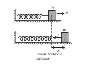
Problem II: universal oscillator

We are dealing with the movement of an object attached to an "ideal spring" (see the figure below). The equation of motion (we use $x$ to denote the position, and $t$ the time) following Hooke's law is $F(t)=mx''(t)=-k(x(t)-x_0)$ , where $k$ is the spring constant and $x_0$ is the position where the spring is not stretched. Here ideal means $k$ is independent of the position. This is impossible in real world.

6. (Harmonic oscillator) Let $x(0) = x_0$ and $x'(0) = v_0$ be the initial conditions, write down the particular solution for $t\ge0$ . What is the period of the movement?

Suppose that $k>0$ . As $x''(t)+\frac{k}{m}x(t)=\frac{kx_0}{m}$ , the general solution of this equation is $x(t)=A\cos(\sqrt\frac{k}{m}t+\phi)+x_0$ . Consider $x(0)=A\cos\phi+x_0=x_0,x'(0)=-A\sqrt\frac{k}{m}\sin\phi=v_0$ , we have $\cos\phi=0,A\sin\phi=-v_0\sqrt\frac{m}{k}$ . So $x(t)=-A\sin\phi\sin\sqrt{\frac{k}{m}}t+x_0=v_0\sqrt\frac{m}{k}\sin\sqrt\frac{k}{m}t+x_0$ . And the period of the movement is $\frac{2\pi}{\sqrt\frac{k}{m}}=2\pi\sqrt\frac{m}{k}$ .

7. (Damped motion) Assume that now there is friction between the object and ground, and the force of friction is proportional to its velocity. Check that the equation of motion is modified to (assume $-2m\eta$ is the constant of the proportionality, $\frac{k}{m}= \omega_0^2$ and $x_0 =0$ ) $F(t) = x''(t) = -2\eta x'(t)-\omega_0^2x(t)$ . Let $x(0) = 0$ and $x'(0) = v_0$ , give the particular solution of the equation.

Assume that $\eta >0$ . Adding the force of friction into $F(t)=mx''(t)=-k(x(t)-x_0)$ , we have $F(t)=mx''(t)=-kx(t)-2m\eta x'(t)$ . As $\frac{k}{m}=\omega_0^2$ , the equation can be written as $x''(t)=-2\eta x'(t)-\omega_0^2x(t)$ .
The eigenvalue equation of $x''(t)=-2\eta x'(t)-\omega_0^2x(t)$ is $\lambda^2+2\eta \lambda+\omega_0^2=0$ . First consider $\eta^2>\omega_0^2$ . $\lambda=-\eta\pm \sqrt{\eta^2-\omega^2_0}$ . So the general solutions of the equation are $x(t)=C_1\exp((-\eta+ \sqrt{\eta^2-\omega^2_0})t)+C_2\exp((-\eta-\sqrt{\eta^2-\omega^2_0})t)$ . Consider $x(0)=C_1+C_2=0,x'(0)=2\sqrt{\eta^2-\omega_0^2}C_1=v_0$ , therefore $C_1=\frac{v_0}{2\sqrt{\eta^2-\omega_0^2}},C_2=-\frac{v_0}{2\sqrt{\eta^2-\omega_0^2}}$ . So the particular solution of the equation is $x(t)=\frac{v_0}{2\sqrt{\eta^2-\omega_0^2}}\exp((-\eta+ \sqrt{\eta^2-\omega^2_0})t)-\frac{v_0}{2\sqrt{\eta^2-\omega_0^2}}\exp((-\eta-\sqrt{\eta^2-\omega^2_0})t)$ . Then consider $\eta^2<\omega_0^2$ . $\lambda=-\eta\pm i\sqrt{\omega^2_0-\eta^2}$ . So the general solutions of the equation are $x(t)=e^{-\eta t}(C_1\cos\sqrt{\omega_0^2-\eta^2}t+C_2\sin\sqrt{\omega_0^2-\eta^2}t)$ . Consider $x(0)=C_1=0,x'(0)=\sqrt{\omega_0^2-\eta^2}C_2=v_0$ , therefore $C_1=0,C_2=\frac{v_0}{\sqrt{\omega_0^2-\eta^2}}$ . So the particular solution of the equation is $x(t)=\frac{v_0}{\sqrt{\omega_0^2-\eta^2}}e^{-\eta t}\sin(\sqrt{\omega_0^2-\eta^2}t)$ .
Combine the two situations, we have $x(t)=\left\{\begin{matrix}\frac{v_0e^{-\eta t}}{2\sqrt{\eta^2-\omega_0^2}}(e^{\sqrt{\eta^2-\omega^2_0}t}-e^{-\sqrt{\eta^2-\omega^2_0}t})&,\eta^2>\omega_0^2 \\ \frac{v_0}{\sqrt{\omega_0^2-\eta^2}}e^{-\eta t}\sin(\sqrt{\omega_0^2-\eta^2}t) &,\eta^2<\omega_0^2\end{matrix}\right.$ .

8. (Forced oscillator) If the object is coupled with an external force (think there is a machine linked to the object), then the model is modified to $x''(t) +2\eta x'(t)+ \omega_0^2x(t) = f(t)$ . First consider the case $\eta= 0$ . Let $f(t) = F \sin( \omega t)$ . Give a particular solution of the equation for i) $\omega\neq\omega_0$ , ii) $\omega=\omega_0$ .

As $\eta=0$ , the equation turns into $x''(t)+\omega_0^2x(t)=F\sin(\omega t)$ .
i) Notice that $x(t)=-\frac{F}{\omega^2-\omega_0^2}\sin(\omega t)$ is a particular solution of the equation.
ii) Notice that $x(t)=-\frac{F}{2\omega_0}t\cos(\omega_0 t)$ is a particular solution of the equation.
(By considering $\lim_{\omega\rightarrow\omega_0}x(t)=-\frac{F}{2\omega_0}\lim_{\omega\rightarrow\omega_0}\frac{\sin(\omega t)}{\omega-\omega_0}=-\frac{F}{2\omega_0}\frac{(\sin(\omega t))_{\omega}}{(\omega-\omega_0)_{\omega}}|_{\omega=\omega_0}=-\frac{F}{2\omega_0}t\cos(\omega_0 t)$ , we can also get the $\omega=\omega_0$ situation. The equation is promised by the uniform continuity of the ODE solutions space.)

9. (Forced damped oscillator) Consider the case $\eta> 0$ and $f(t) = F \sin( \omega t +\beta )$ . The equation of motion is now $x''(t) +2\eta x'(t)+ \omega_0^2x(t) = F \sin( \omega t+\beta )$ . Give a particular solution of the equation.

Consider $\omega\neq\omega_0$ , notice that $x(t)=\frac{F\cos(\omega t+\beta+\arctan\frac{\omega^2-\omega_0^2}{2\eta\omega})}{\sqrt{(\omega^2-\omega_0^2)^2+4\eta^2\omega^2}}$ is a particular solution of the equation.
When $\omega=\omega_0$ , let $\omega\rightarrow\omega_0$ . We have $x(t)=\frac{F}{2\eta\omega_0}\cos(\omega_0 t+\beta)$ is a particular solution of the equation.

10. Give the general solution of the equation. As $t\rightarrow\infty$ , try to illustrate the movement of the object.

Combine 7. and 9., we have $x(t)=\left\{\begin{matrix}\frac{v_0e^{-\eta t}}{2\sqrt{\eta^2-\omega_0^2}}(e^{\sqrt{\eta^2-\omega^2_0}t}-e^{-\sqrt{\eta^2-\omega^2_0}t})+\frac{F\cos(\omega t+\beta+\arctan\frac{\omega^2-\omega_0^2}{2\eta\omega})}{\sqrt{(\omega^2-\omega_0^2)^2+4\eta^2\omega^2}} &,\eta^2>\omega_0^2 \\ \frac{v_0}{\sqrt{\omega_0^2-\eta^2}}e^{-\eta t}\sin(\sqrt{\omega_0^2-\eta^2}t) +\frac{F\cos(\omega t+\beta+\arctan\frac{\omega^2-\omega_0^2}{2\eta\omega})}{\sqrt{(\omega^2-\omega_0^2)^2+4\eta^2\omega^2}}&,\eta^2<\omega_0^2\end{matrix}\right.$ .
When $t\rightarrow\infty$ , the terms $e^{(-\eta+\sqrt{\eta^2-\omega_0^2})t},e^{(-\eta-\sqrt{\eta^2-\omega_0^2})t},e^{-\eta t}\rightarrow 0$ , which means $x(t)\rightarrow\frac{F\cos(\omega t+\beta+\arctan\frac{\omega^2-\omega_0^2}{2\eta\omega})}{\sqrt{(\omega^2-\omega_0^2)^2+4\eta^2\omega^2}}$ . So the graph of the movement of the object when $t\rightarrow\infty$ is same as the graph of $x(t)=\frac{F\cos(\omega t+\beta+\arctan\frac{\omega^2-\omega_0^2}{2\eta\omega})}{\sqrt{(\omega^2-\omega_0^2)^2+4\eta^2\omega^2}}$ .